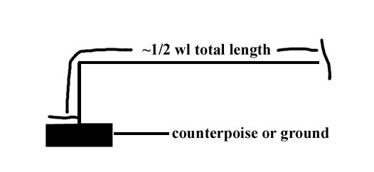
End-fed 1/2 wave parallel resonant feed system end feed
|
|
End Fed Half
|
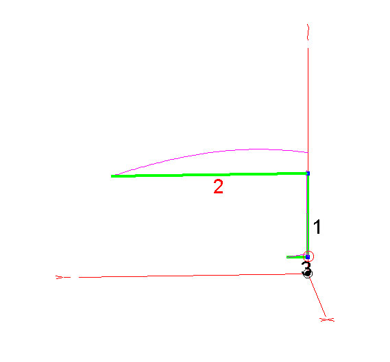
| Note: The very small difference in apparent currents in the counterpoise and antenna at their junction is caused by the counterpoise being short. The short counterpoise has a very rapid reduction in current along its length. Eznec gives the mean current over the length of a segment, not the segment entrance or exit current. This means the high current taper makes the average current along the length of a segment appear to be less. |
One recently
proposed theory is
this; “if the
antenna is not
exactly resonant,
ground currents will
flow.” We
already know ground
currents flow with a
resonant end-fed
because
end-impedance is not
infinite. Let’s
change frequency
10%, since this
would be equivalent
to a 10% error in
length of all
sections, and
see how much ground
currents increase…
EFHW standard
6/3/05 5:43:47 PM
—————
CURRENT DATA
—————Frequency
= 7.788 MHz
lowest vertical
antenna
segment .37542
counterpoise first
segment
.35496a
Before at
resonance we had:
lowest vertical
antenna segment
.17408a
counterpoise
first
segment
.16418a
Being 10% off
resonance just about
doubles current. We
see it is a definite
current increase,
but not one from
zero to problematic
currents! The
proposal exact
resonance eliminates
all current in a
counterpoise isn’t
correct. A 10%
length error only
doubles
current.
Moving 5% in
frequency:
EFHW standard
6/3/05 6:20:14 PM
—————
CURRENT DATA
—————Frequency
= 7.434 MHz
lowest vertical
antenna
segment
.2049
counterpoise first
segment
.19385
| Note: The very small difference in apparent currents in the counterpoise and antenna at their junction is caused by the counterpoise being short. The short counterpoise has a very rapid reduction in current along its length. Eznec gives the mean current over the length of a segment, not the segment entrance or exit current. This means the high current taper makes the average current along the length of a segment appear to be less. |
With a 5% length
error from
resonance, we now
see only an 18%
increase in current.
That’s negligible
since many other
things we might do
(like moving the
antenna a few feet
in height) would
make a much larger
change.
—————
SOURCE DATA
—————Frequency
= 7.434 MHz
Source 1 Voltage =
924.9 V. at -58.15
deg.
Current = 0.2049 A.
at 0.0 deg.
Impedance = 2382 – J
3834 ohms
Power = 100 watts
We can see there
is some merit to
maintaining
resonance because
current is at a
minimum value, but
we only need to
worry when resonance
errors are somewhat
large. When length
errors are modest
(under 5%) the error
has virtually no
effect on ground
current. The reason
for this is very
simple. The
reactance or lack of
resonance isn’t what
determines current,
the resistive part
of the impedance
does. We are looking
for a resistance
peak in the
end-impedance of the
antenna…not
necessarily
resonance.
The source resistive
part at resonance
was 3300 ohms. At 5%
error it was 2382
ohms.
With the
non-resonant
antenna, we have
increased electric
fields around the
feedpoint. Voltage
is 925v instead of
575 volts. RF
voltages (the
electric field)
might be an issue
with end-fed
antennas.
What else
affects Antenna
Impedance?
From above we see
higher antenna
resistance is a good
thing for current,
and length is not
overly critical. We
also see lower
reactance is a good
thing for voltage,
and length can
affect voltages (and
the electric field)
surrounding the
antenna and
counterpoise near
the feedpoint.
What about
a thicker antenna?
With a 1″ thick
antenna 7 MHz
impedance becomes
1684 – J 716.3 ohms
and resonance is
well below 6 MHz.
The reactance
problem is because
the counterpoise is
too short. The
drastic resistance
reduction at peak
resistance occurs
because the wire is
thicker. Obviously a
thicker antenna has
higher ground
currents!
Half-wave
broadcast towers
often have
impedances under 800
ohms at
resonance.
What about
antenna
surroundings? As
the area around the
antenna becomes more
cluttered and/or has
more power loss,
antenna
end-resistance is
reduced! Over
perfect ground the
antenna
end-impedance almost
doubles from that
over average ground.
Over lossy ground,
especially when the
antenna is low in
height, feed
resistance decreases
even more.
With a
small counterpoise
and end-feed
we:
- need to
keep the antenna
clear of lossy
media including
the earth. - should try
to use a
reasonably thin
antenna element
to minimize
current. - stay within
a few percent of
resonance to
minimize
feedpoint
voltage and
current. - always have
the same current
flowing into a
counterpoise (of
some form) as
flows into the
antenna. - should use
the largest
counterpoise
that can be
reasonably
implemented, but
avoid small
counterpoise
systems that
have wires
significantly
longer than 1/4
wl
Improvements
The best solution
I can think of to
common mode or
“RF in the
shack” problems
with this form of
antenna is to
isolate the
counterpoise or
antenna ground from
the station feed. At
low power levels a
simple link coupled
matching network is
a good solution,
provided the
secondary has no RF
path to station
equipment. One way
to accomplish this
is by using two
output terminals
that float.
In the circuit
above:
- Determine the
maximum
impedance ratio
between input
and
output. - The turns
ratio is the
square root of
that ratio - The reactance
value of C1 near
3/4 mesh at the
lowest frequency
and secondary
reactance of T1
should be the
maximum expected
load impedance
over the turns
ratio - C2 is
optional, and
should be the
value of C1 or
larger if used.
It will allow
wide adjustment
of matching
range
Assume we have a
5000 ohm load and 50
ohm rig. The turns
ratio of T1 is sqrt
of 5000/50 or a 10:1
ratio.
The reactance of
C1 at 3/4 mesh (so
you have adjustment
range) should be
5000/10, or 500
ohms. (This is a
loaded Q of ten, you
need LESS Q with
lower transformation
ratios and more Q
with higher ratios
or the circuit
becomes too sharp or
too
“mushy” to
tune.)
The reactance of
L1 secondary should
be 500 ohms in this
example.
U1 should connect
to the antenna, U2
to the counterpoise
or ground which
should NOT connect
to the station
equipment. The
counterpoise should
be as long and
straight as
possible, and
directly under the
antenna if possible.
Ideally the
counterpoise, if
less than 8 wires
1/4 wl long, should
be elevated and
insulated from
earth. Do NOT
make the
counterpoise longer
than 1/4 wl,
especially if it is
only a single wire! Most
of us, since this is
a temporary or
compromise antenna,
will use a very
small ground system.
I’ve found
connecting a
counterpoise to
earth, say a ground
rod, actually
reduces antenna
efficiency.
If you run low
power and don’t have
a ground or
counterpoise, you
might just connect
U2 right back to the
coax shield from the
radio. This way you
can use the
capacitance of the
radio and station
wiring as a ground
system.
To
be continued soon!
Zepp or stub-matched
antenna
Dipole with coax
having a choke at
the end
Impedance
Feed Systems
Common Mode
Currents
Modified
June 1, 2005 more
data being added
over the next few
days…
At high power 3
dB loss in even the
largest components
would mean extreme
heat, at low power
its difficult to
notice several dB
loss as any type of
component heating.
The paradox is while
1500 watt systems
could often stand to
lose 10 dB or more
as heat…low power
systems (at least in
my way of thinking)
should try to
squeeze every
milliwatt out!
Let’s look at a
matching system in
what I consider one
of the most
difficult methods of
feeding an antenna,
the end fed
half-wave. If anyone
has any other
matching systems
that are commonly
used or recommended,
send me one and I’ll
measure it in my
lab and post the
data
here.
There is also
some discussion of
common mode current,
and the lack of
common mode current
because we sometimes
can’t observe ill
effects.
I remember
working with a new
graduate engineer,
let’s call him
Simon, on an antenna
system. When I asked
Simon if he checked
for proper feedpoint
isolation, he turned
an SWR analyzer on
and wrapped his
fingers around the
feed line. Seeing no
change in SWR, he
declared the system
free of common mode
currents! Convincing
him to use a clamp-on
RF meter, we
found the feed line
that acted
“cold” to
the touch actually
had significant
common mode
currents.
Where did Simon
go wrong? Pretty
simple when we think
about what he was
actually testing.
High voltage points
interact with body
capacitance at HF,
not current points!
Had Simon grabbed
the coax at a high
voltage point of the
shield, he might
have found
interaction with
SWR. Unfortunately a
significantly high
impedance or high
voltage point rarely
appears along the
outside of a
“grounded”
shield. That’s
because the cable is
often routed near
other conductors.
The cable is also
thick, and that
limits surge
impedance.
Even if we modify
common mode
impedance with body
capacity, the
feedpoint is where
multiple paths
combine and make the
transition to the
feed line. Measuring
SWR changes is a
very poor way to
determine proper
operation. Even the
most basic antenna
systems, once the
feed line becomes
involved, can become
a terribly complex
web of paths. The
myth that we can
grab a cable to see
if a system needs a
balun or has common
mode problems is a
very BIG
myth.
End-fed Matching
Circuit
Measurement
In order to
quantify efficiency
of a typical
matching system, I
made a concerted
effort to duplicate
the coupler
AA5TB describes on his
web page. (I
think the basic
AA5TB system is a
good one, but I’d
probably make a few
changes.)
I used the same
wire gauge, core
type and material,
same turns ratio,
and a very similar
brand new capacitor
of the same
construction and
style for
measurements below.
The measurements
below are on
equipment certified
to national
standards. The
primary instrument
is a HP-8753E
network analyzer,
and was verified by
a HP-4191A
laboratory standard
impedance test set.
Here is an
impedance sweep of
the parallel tuned
network, adjusted to
the upper end of 40
meters. AA5TB has it
at http://webpages.charter.net/aa5tb/coupler2.html
You can see,
despite claims the
antenna is ground
independent, the
secondary is
connected
to…..ground.
Actually I can
eliminate that
ground connection
and, by increasing
the transformer
turns ratio, still
feed the antenna!
How is it possible
to feed a single
terminal with
current? Simple. The
hanging end of the
winding will
capacitively couple
to ground and
provide a path for
return currents. We
can’t get away from
it, an end-fed wire
is NOT a dipole. The
feed line and
everything connected
to the feed line
becomes the return
path for
displacement
currents. It always
has, it always will.
The common mode
feed line and antenna
currents, at the
matching system,
will always be
equal. The same
common mode current
will leave on the
shield as pushes up
into the antenna,
the only exception
is if the matching
system is physically
large compared to
the antenna and the
matching system by
itself becomes a
groundplane.
Remember I made a
best effort to
duplicate the
matching system. The
measured data
follows:
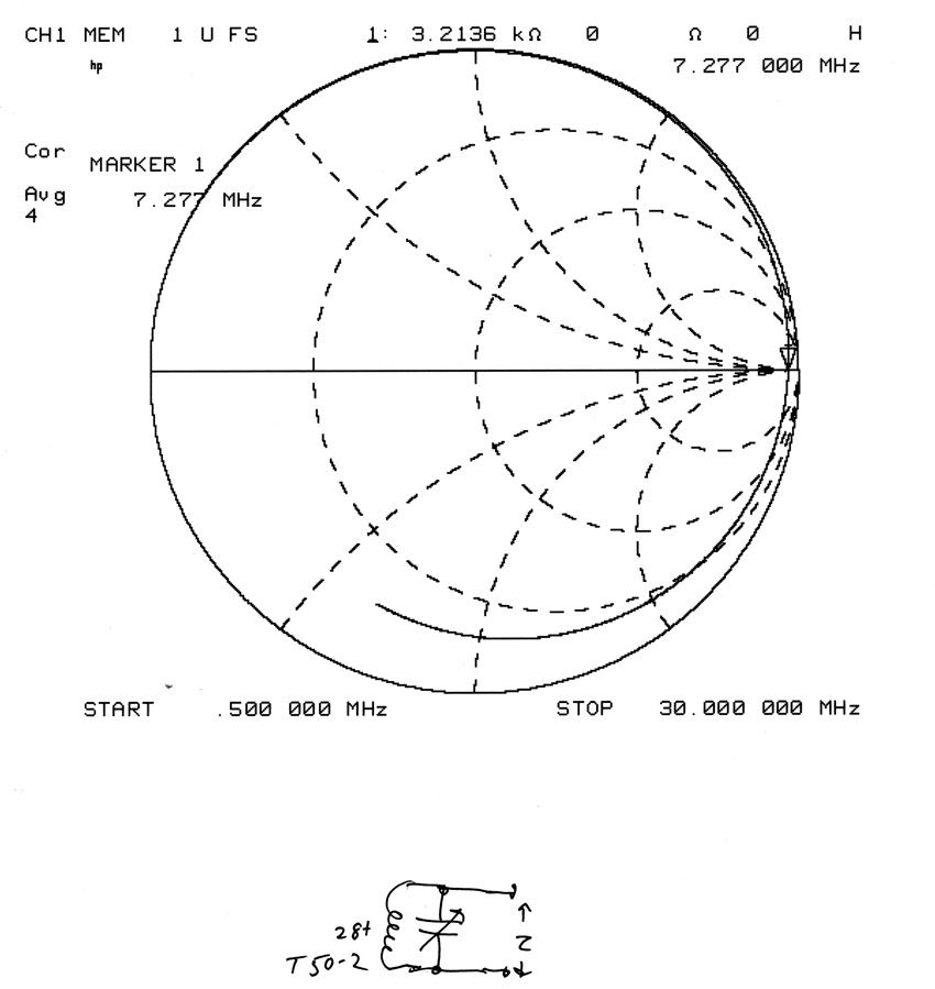
You can see from
the data above, with
no load on the
primary or
secondary, this
parallel resonant
circuit looks like
3.2k ohms (J0 at
resonance) at 7
MHz.
3.2k ohms is the
equivalent parallel
(or shunting)
resistance across
the load. This
resistance is caused
by losses in the
inductor, the
variable capacitor,
and some very small
wiring resistances.
Losses actually
break down this way:
Inductor measured
Q =
78
@ L =
4.12 uH
Capacitor
measured Q =
22.8 @
C=118.7 pF
Reactance was
186.2 ohms
While the
inductor had what I
consider poor Q, the
capacitor was a real
killer. It was a
brand new capacitor
from stock of sample
parts. Four more
tested similarly,
with the highest Q
of the five only
38.5! The
manufacturer was
Apollo
The only other
miniature capacitor
I had of similar
construction to the
one AA5TB used was a
Taiwanese capacitor
with the logo
“OM”. This
batch was another
group of sample
parts. In this case
capacitor Q at 118.7
pF ranged from 38.0
to 43.2. This is
still very low Q.
The parallel
resistance
representing
losses was 4.9
k ohms, up from 3.2
k ohms using the OM
capacitors.
The final test
was an air variable.
The air variable was
a standard compact
receiving type 140
pF capacitor
manufactured by Oren
Elliot Products (All
Star Products) in
Edgerton, Ohio. In
this case capacitor
Q measured 2565!!
That Q is roughly
100 times the Apollo
capacitor Q. I only
measured a sample of
one capacitor.
Using this
capacitor with no
other changes, the
parallel resistance
of the above circuit
was around 20,000
ohms.
Efficiency Table
The table below
used 5 watts applied
power and a 4700 ohm
load.
| Capacitor | Cap RMS Voltage |
Power at load |
Power lost |
% eff |
Loss |
| Apollo Series |
98.5 | 2.07 W |
2.93 W |
41.4 % |
-3.8 dB |
| OM series |
109.6 | 2.56 W |
2.44 W |
51.2 % |
-2.9 dB |
| Air Variable |
132.8 | 3.75 W |
1.25 W |
75 % |
-1.2 dB |
Of particular
concern is the low Q
of compact
capacitors as well
as upper impedance
limits of compact
powdered iron cores
wound with large
numbers of
turns. It would
be much better to
use a small air
variable rather
than
notoriously
troublesome
“transistor
radio” tuning
capacitors.
The inductor
could also be
improved with a
taller core or stack
of cores. That would
minimize the number
of turns required
for resonance! Also
a different mix
might increase Q.
On the previous
page, I mentioned
the impedance ratio
of a tightly coupled
transformer of high
quality was equal to
the square of the
turns ratio between
primary and
secondary. If we
wanted to match a
4700 ohm load to a
50 ohm source, the
turns ratio should
be sqrt of 4700/50,
or 9.7 : 1.
4700 in parallel
with 3300 is 1939
ohms. 1939 ohms over
50 ohms is a
resistance ratio of
38.78. The square
root of 38.78 is
6.23. 28/6.23 is 4.5
turns. I calculate a
4.5 turn primary
based on perfect
mutual coupling, the
3.3k secondary loss
equivalent parallel
resistance, 4700 ohm
load, and a 28-turn
secondary.
4.5 turns isn’t
possible, and won’t
be exact anyway
because of flux
leakage, lead
lengths, and other
small imperfections
in the system. The
plot below is with a
5 turn
primary.
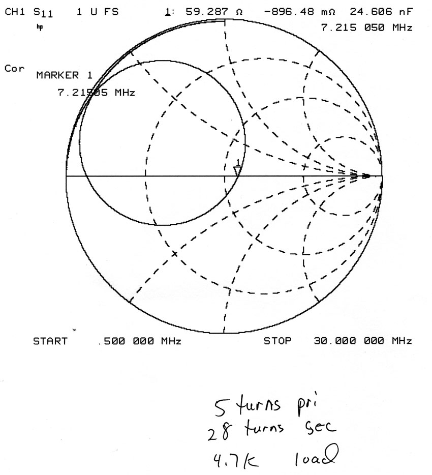
Let’s work the
problem backwards.
The 28 turn
secondary / 5 turn
primary transformer
I measured above has
a turns ratio of
5.6:1
5.6 squared is
31.36
The measured primary
impedance was 62 j0,
times the impedance
ratio of 31.36, for
a net secondary
impedance of
31.36*62 = 1944
ohms. That isn’t
terribly far from
the 1939 ohms
calculated as 3300
ohms of tank
parallel equivalent
loss resistance in
parallel with 4700
ohms of load
resistance!
Measuring things
two different ways
and comparing
results is very
useful. It warns us
of any errors in
measurements, logic,
or misapplications
of theory.
When I measured
the secondary
impedance, I
calculated I’d need
about 4.5 turns on
the primary to match
a 4700 ohm load in
parallel with a loss
resistance of 3300
ohms, or 1939 ohms.
When I optimized the
transformer, I found
5 turns was close
enough.
So there we have
it. Matching loss in
the worse
transformer system I
measured is around 4
dB. If the antenna
was 4700 ohms j0,
more power would be
consumed in the tank
circuit feeding the
antenna than is
actually applied to
the radiating part
of the antenna
system! Of the power
applied to the
antenna, a
significant portion
will be distributed
in the antenna feed
cables, rig, and
everything connected
to the rig including
the operator and
station wiring.
On the other hand
we could build a
dipole, and feed it
with RG-174 cable.
We would eliminate
about 4 dB of
matching circuit
losses, and a few dB
of power lost in
common mode losses.
How much RG-174
could we use to
equal the end-fed
losses? At 50 MHz we
could use about
100-feet of RG-174
and break even with
end feed using the
system I
constructed, a small
T50-2 toroid with
link coupling
resonated by a
typical polyethylene
insulated
“broadcast
tuning”
capacitor. At 7 MHz
it’s a no-brainer.
I’ll take the RG-174
dipole feed every
time! My
reasons are mostly
the convenience and
repeatability of the
feed system.
Another possible
alternative is a 1/4
wl 450-ohm Q section
or stub. TLA
estimates loss as
.205dB on 7 MHz with
that system.
In my experience
it’s far easier to
have repeatable
results with a stub,
rather than small
inconsistently
manufactured lumped
networks. Even large
tuners using
transmitting
components become
inconsistent in loss
measurements at
impedance extremes.
Losses that would
cause big smoke at
high power can go
unnoticed at low
power
levels..
End-fed half
waves are sometimes
inefficient or
troublesome feed
systems. At low
power we might
never notice
efficiency problems
or common mode
current problems. Of
course at high power
very few shortcuts
can be tolerated.
as
of 5/27/2005
This page
copyright W8JI 2005.
All drawings and
text may be used
when discussing
specifics of this
article (that’s fair
use), but may not be
used in any other
form.